How do I change maximum axis value?

How do I change maximum axis value?

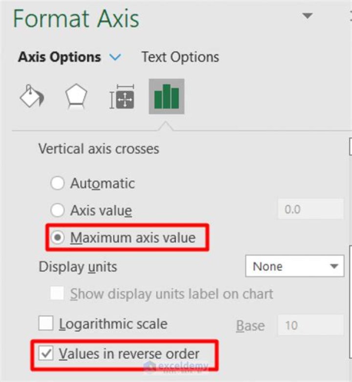
Here is a better way to change the automatic axis settings:

1. Open the Excel file containing the chart.
2. Click a value in the chart’s vertical axis to select it.
3. Right-click the selected vertical axis.
4. Click Format Axis.
5. Click the Fixed button for Minimum.
6. Click the Fixed button for Maximum.

How do you set a maximum value in an Excel graph?

Select the chart series and go to format series (Click on the series, press CTRL+1). Now, set up series overlap to 100% and your maximum value is highlighted. That is all. In just a few minutes and clicks, your chart highlights maximum value.

How do you change the axis range in Excel?

How to Change the X-Axis Range

1. Open the Excel file with the chart you want to adjust.
2. Right-click the X-axis in the chart you want to change.
3. Then, click on Select Data.
4. Select Edit right below the Horizontal Axis Labels tab.
5. Next, click on Select Range.

How do you set a maximum value in a graph?

Double-click your chart to edit it. Click the Settings gear in the top right corner of the chart pop-up window. Enter the minimum and/or maximum y-axis/x-axis value for your chart.

How do I change the y axis values in Excel?

Click the chart, and then click the Chart Layout tab. Under Axes, click Axes > Vertical Axis, and then click the kind of axis label that you want.

How do I create a clustered combo chart in Excel?

To create a combination chart, execute the following steps.

1. On the Insert tab, in the Charts group, click the Combo symbol.
2. Click Create Custom Combo Chart.
3. The Insert Chart dialog box appears. For the Rainy Days series, choose Clustered Column as the chart type.
4. Click OK. Result:

How do you find the maximum value in Excel?

Calculate the smallest or largest number in a range

1. Select a cell below or to the right of the numbers for which you want to find the smallest number.
2. On the Home tab, in the Editing group, click the arrow next to AutoSum. , click Min (calculates the smallest) or Max (calculates the largest), and then press ENTER.

How do I create a dynamic axis in Excel?

The steps to add an axis title to a dynamic chart in Excel are as follows: 1 – Select the chart and in the Design tab, go to Chart Layouts. 2 – Open the drop-down menu under “Add Chart Element.” In the earlier versions of Excel, go to “labels” in the Layout tab and click on “axis title.”

How do you find the maximum and minimum of a graph in Excel?

Right click on the Max point, and choose Data Labels. Select the label and choose the Series Name option, so it shows “Max”, and choose the bright blue text color. Format the marker so it’s an 8-point circle with a 1.5-pt matching blue border and no fill. Right click on the Min point, and choose Data Labels.

How do I change axis value to text in Excel?

Change axis labels in a chart

1. Click each cell in the worksheet that contains the label text you want to change.
2. Type the text you want in each cell, and press Enter. As you change the text in the cells, the labels in the chart are updated.

How do you define maximum data BAR values?

Data Bar Maximum

1. Open the Edit Rule dialog box.
2. For Maximum, click the Type arrow, and choose Formula.
3. In the Value box, type this formula: =MAX($G$4:$G$9)*1.3.

How do I add a secondary axis in Excel?

Add or remove a secondary axis in a chart in Excel

1. Select a chart to open Chart Tools.
2. Select Design > Change Chart Type.
3. Select Combo > Cluster Column – Line on Secondary Axis.
4. Select Secondary Axis for the data series you want to show.
5. Select the drop-down arrow and choose Line.
6. Select OK.